In-class Exercise 2: Geospatial Data Wrangling with R

Published

January 16, 2023

Modified

February 8, 2023

Installing the R packages

First, we need to check if we have the three R packages to be used for the In-Class Excercise (sf ,tidyverse and funModelling) installed. If not, we need to install it automatically. The below code checks if the packages are already installed, else it will install the packages for us. However, before running the below code, ensure that ‘packman’ package has been installed in your RStudio.

pacman::p_load(sf, tidyverse, funModeling)

Importing the Geospatial Dataset

The geoBoundaries Dataset

To Import the Geospatial data, run the following code. Ensure that the directory of the files and the file name is correct. By running the code, the data will be in meters and it will be in simple feature format.

geoNGA <- st_read("data/geospatial", 
                  layer = "geoBoundaries-NGA-ADM2") %>%
  st_transform(crs = 26392)

Reading layer `geoBoundaries-NGA-ADM2' from data source 
  `C:\mayurims\IS415-GAA\In-Class_Ex\In-Class_Ex02\data\geospatial' 
  using driver `ESRI Shapefile'
Simple feature collection with 774 features and 6 fields
Geometry type: MULTIPOLYGON
Dimension:     XY
Bounding box:  xmin: 2.668534 ymin: 4.273007 xmax: 14.67882 ymax: 13.89442
Geodetic CRS:  WGS 84

Importing the NGA Dataset

To Import the NGAdata, run the following code. Ensure that the directory of the files and the file name is correct.

NGA <- st_read("data/geospatial", 
                  layer = "nga_admbnda_adm2_osgof_20190417") %>%
  st_transform(crs = 26392)

Reading layer `nga_admbnda_adm2_osgof_20190417' from data source 
  `C:\mayurims\IS415-GAA\In-Class_Ex\In-Class_Ex02\data\geospatial' 
  using driver `ESRI Shapefile'
Simple feature collection with 774 features and 16 fields
Geometry type: MULTIPOLYGON
Dimension:     XY
Bounding box:  xmin: 2.668534 ymin: 4.273007 xmax: 14.67882 ymax: 13.89442
Geodetic CRS:  WGS 84

Importing Aspatial data

Similar to the Geospatial data, import the Aspatial data, however, remember that the data is in CSV format and hence, read_csv() must be used

wp_nga <- read_csv("data/aspatial/WPdx.csv") %>%
  filter(`#clean_country_name` == "Nigeria")

Converting Aspatial Data into Geospatial

We now convert the newly extracted Aspatial data (wp_nga) into point sf dataframe using the below code.

wp_nga$Geometry = st_as_sfc(wp_nga$`New Georeferenced Column`)
wp_nga

# A tibble: 95,008 × 71
   row_id `#source`      #lat_…¹ #lon_…² #repo…³ #stat…⁴ #wate…⁵ #wate…⁶ #wate…⁷
    <dbl> <chr>            <dbl>   <dbl> <chr>   <chr>   <chr>   <chr>   <chr>  
 1 429068 GRID3             7.98    5.12 08/29/… Unknown <NA>    <NA>    Tapsta…
 2 222071 Federal Minis…    6.96    3.60 08/16/… Yes     Boreho… Well    Mechan…
 3 160612 WaterAid          6.49    7.93 12/04/… Yes     Boreho… Well    Hand P…
 4 160669 WaterAid          6.73    7.65 12/04/… Yes     Boreho… Well    <NA>   
 5 160642 WaterAid          6.78    7.66 12/04/… Yes     Boreho… Well    Hand P…
 6 160628 WaterAid          6.96    7.78 12/04/… Yes     Boreho… Well    Hand P…
 7 160632 WaterAid          7.02    7.84 12/04/… Yes     Boreho… Well    Hand P…
 8 642747 Living Water …    7.33    8.98 10/03/… Yes     Boreho… Well    Mechan…
 9 642456 Living Water …    7.17    9.11 10/03/… Yes     Boreho… Well    Hand P…
10 641347 Living Water …    7.20    9.22 03/28/… Yes     Boreho… Well    Hand P…
# … with 94,998 more rows, 62 more variables: `#water_tech_category` <chr>,
#   `#facility_type` <chr>, `#clean_country_name` <chr>, `#clean_adm1` <chr>,
#   `#clean_adm2` <chr>, `#clean_adm3` <chr>, `#clean_adm4` <chr>,
#   `#install_year` <dbl>, `#installer` <chr>, `#rehab_year` <lgl>,
#   `#rehabilitator` <lgl>, `#management_clean` <chr>, `#status_clean` <chr>,
#   `#pay` <chr>, `#fecal_coliform_presence` <chr>,
#   `#fecal_coliform_value` <dbl>, `#subjective_quality` <chr>, …

wp_sf <- st_sf(wp_nga, crs=4326)
wp_sf

Simple feature collection with 95008 features and 70 fields
Geometry type: POINT
Dimension:     XY
Bounding box:  xmin: 2.707441 ymin: 4.301812 xmax: 14.21828 ymax: 13.86568
Geodetic CRS:  WGS 84
# A tibble: 95,008 × 71
   row_id `#source`      #lat_…¹ #lon_…² #repo…³ #stat…⁴ #wate…⁵ #wate…⁶ #wate…⁷
 *  <dbl> <chr>            <dbl>   <dbl> <chr>   <chr>   <chr>   <chr>   <chr>  
 1 429068 GRID3             7.98    5.12 08/29/… Unknown <NA>    <NA>    Tapsta…
 2 222071 Federal Minis…    6.96    3.60 08/16/… Yes     Boreho… Well    Mechan…
 3 160612 WaterAid          6.49    7.93 12/04/… Yes     Boreho… Well    Hand P…
 4 160669 WaterAid          6.73    7.65 12/04/… Yes     Boreho… Well    <NA>   
 5 160642 WaterAid          6.78    7.66 12/04/… Yes     Boreho… Well    Hand P…
 6 160628 WaterAid          6.96    7.78 12/04/… Yes     Boreho… Well    Hand P…
 7 160632 WaterAid          7.02    7.84 12/04/… Yes     Boreho… Well    Hand P…
 8 642747 Living Water …    7.33    8.98 10/03/… Yes     Boreho… Well    Mechan…
 9 642456 Living Water …    7.17    9.11 10/03/… Yes     Boreho… Well    Hand P…
10 641347 Living Water …    7.20    9.22 03/28/… Yes     Boreho… Well    Hand P…
# … with 94,998 more rows, 62 more variables: `#water_tech_category` <chr>,
#   `#facility_type` <chr>, `#clean_country_name` <chr>, `#clean_adm1` <chr>,
#   `#clean_adm2` <chr>, `#clean_adm3` <chr>, `#clean_adm4` <chr>,
#   `#install_year` <dbl>, `#installer` <chr>, `#rehab_year` <lgl>,
#   `#rehabilitator` <lgl>, `#management_clean` <chr>, `#status_clean` <chr>,
#   `#pay` <chr>, `#fecal_coliform_presence` <chr>,
#   `#fecal_coliform_value` <dbl>, `#subjective_quality` <chr>, …

Project Transformation

We now transform the projection from wgs84 to appropriate projected coordinate system of Nigeria.

wp_sf <- wp_sf %>%
  st_transform(crs = 26392)

Geospatial Data Cleaning

Excluding redundent fields

NGA <- NGA %>%
  select(c(3:4,8:9))

Checking for duplicate name

It is important to check for duplicate name in the data main data fields. Using duplicate(), we can flag out the LGA names.

NGA$ADM2_EN[duplicated(NGA$ADM2_EN)==TRUE]

[1] "Bassa"    "Ifelodun" "Irepodun" "Nasarawa" "Obi"      "Surulere"

The printout above shows that there are 6 LGAs with the same name,. A Google search using the coordinates showed that there are LGAs with the same name but are located in different states.

NGA$ADM2_EN[94] <- "Bassa, Kogi"
NGA$ADM2_EN[95] <- "Bassa, Plateau"
NGA$ADM2_EN[304] <- "Ifelodun, Kwara"
NGA$ADM2_EN[305] <- "Ifelodun, Osun"
NGA$ADM2_EN[355] <- "Irepodun, Kwara"
NGA$ADM2_EN[356] <- "Irepodun, Osun"
NGA$ADM2_EN[519] <- "Nasarawa, Kano"
NGA$ADM2_EN[520] <- "Nasarawa, Nasarawa"
NGA$ADM2_EN[546] <- "Obi, Benue"
NGA$ADM2_EN[547] <- "Obi, Nasarawa"
NGA$ADM2_EN[693] <- "Surulere, Lagos"
NGA$ADM2_EN[694] <- "Surulere, Oyo"

Check if there are any duplicated codes now

NGA$ADM2_EN[duplicated(NGA$ADM2_EN)==TRUE]

character(0)

Data Wrangling for Water Point Data

freq(data = wp_sf,
     input = '#status_clean')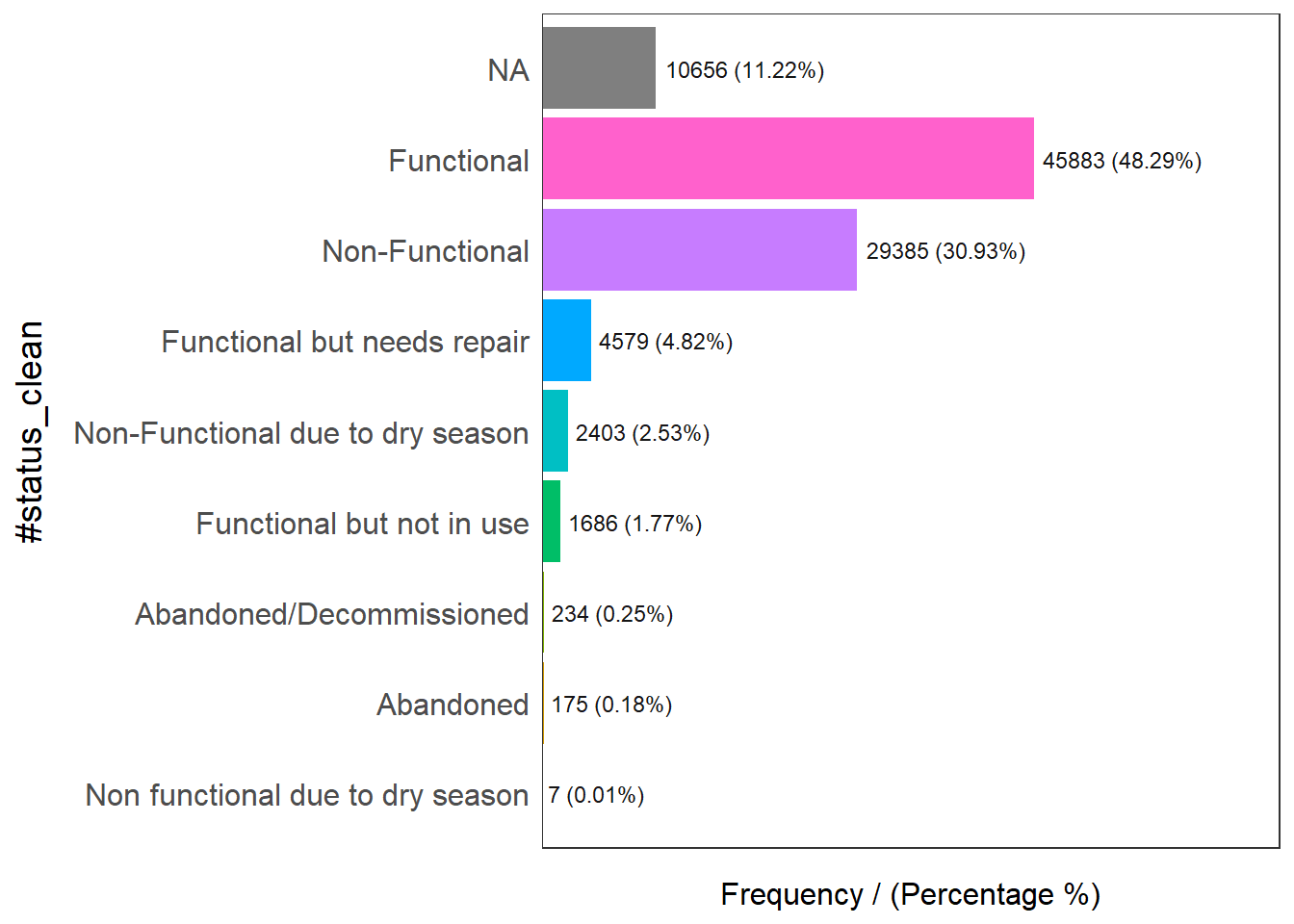

                     #status_clean frequency percentage cumulative_perc
1                       Functional     45883      48.29           48.29
2                   Non-Functional     29385      30.93           79.22
3                             <NA>     10656      11.22           90.44
4      Functional but needs repair      4579       4.82           95.26
5 Non-Functional due to dry season      2403       2.53           97.79
6        Functional but not in use      1686       1.77           99.56
7         Abandoned/Decommissioned       234       0.25           99.81
8                        Abandoned       175       0.18           99.99
9 Non functional due to dry season         7       0.01          100.00

wp_sf_nga <- wp_sf %>%
  rename(status_clean = '#status_clean') %>%
  select(status_clean) %>%
  mutate(status_clean = replace_na(
    status_clean, "unknown"))

Extracting Water Point Data

wp_functional <- wp_sf_nga %>%
  filter(status_clean %in%
           c("Functional",
             "Functional but not in use",
             "Functional but needs repair"))

wp_nonfunctional <- wp_sf_nga %>%
  filter(status_clean %in%
           c("Abandoned/Decommissioned",
             "Abandoned",
             "Non-Functional due to dry season",
             "Non-Functional",
             "Non functional due to dry season"))

wp_unknown <- wp_sf_nga %>%
  filter(status_clean == "unknown")

Next, the code chunk below is used to perform a quick EDA on the derived sf data.frames.

freq(data = wp_functional,
     input = 'status_clean')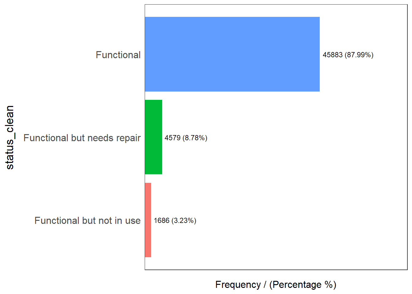

                 status_clean frequency percentage cumulative_perc
1                  Functional     45883      87.99           87.99
2 Functional but needs repair      4579       8.78           96.77
3   Functional but not in use      1686       3.23          100.00

freq(data = wp_nonfunctional,
     input = 'status_clean')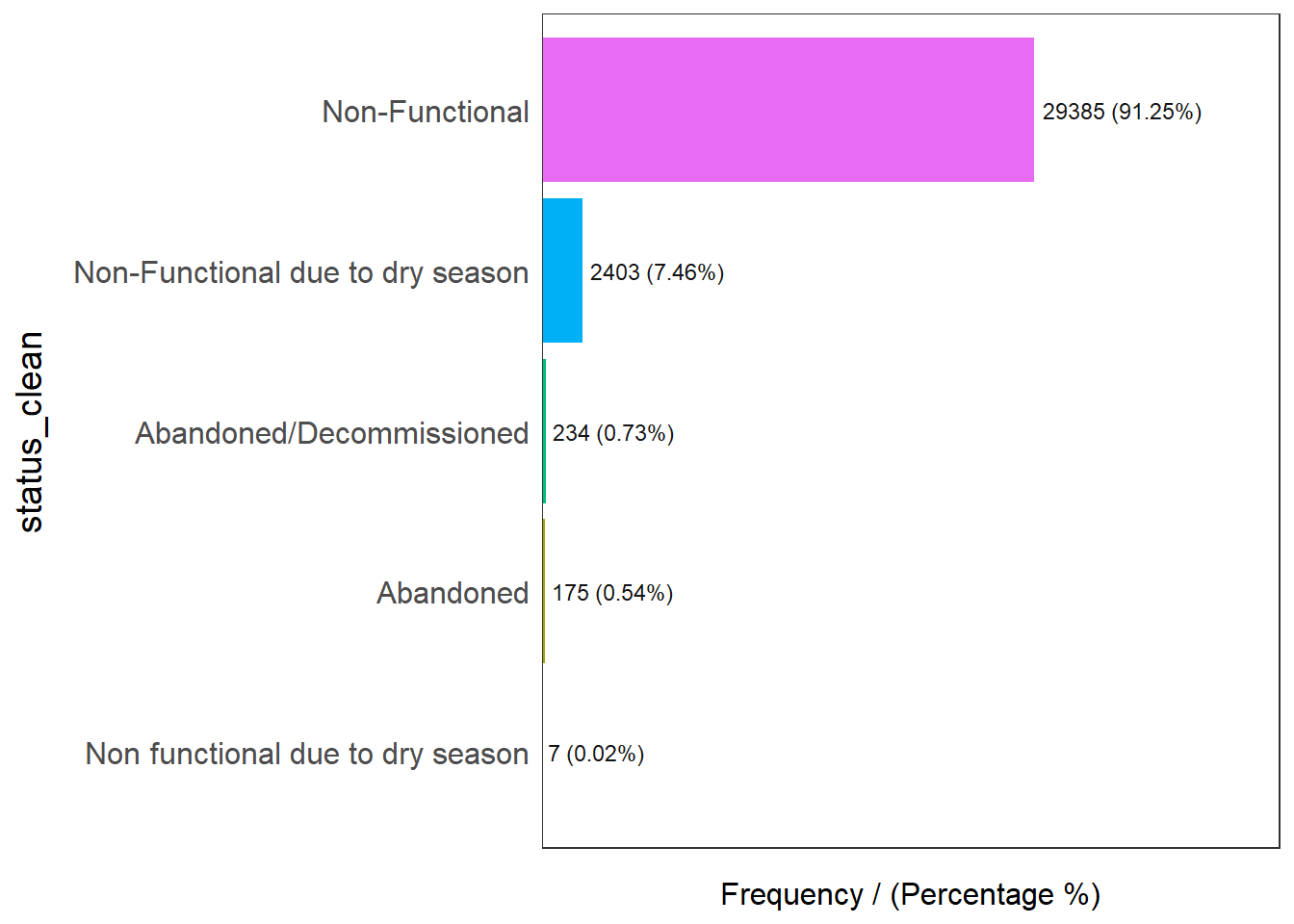

                      status_clean frequency percentage cumulative_perc
1                   Non-Functional     29385      91.25           91.25
2 Non-Functional due to dry season      2403       7.46           98.71
3         Abandoned/Decommissioned       234       0.73           99.44
4                        Abandoned       175       0.54           99.98
5 Non functional due to dry season         7       0.02          100.00

freq(data = wp_unknown,
     input = 'status_clean')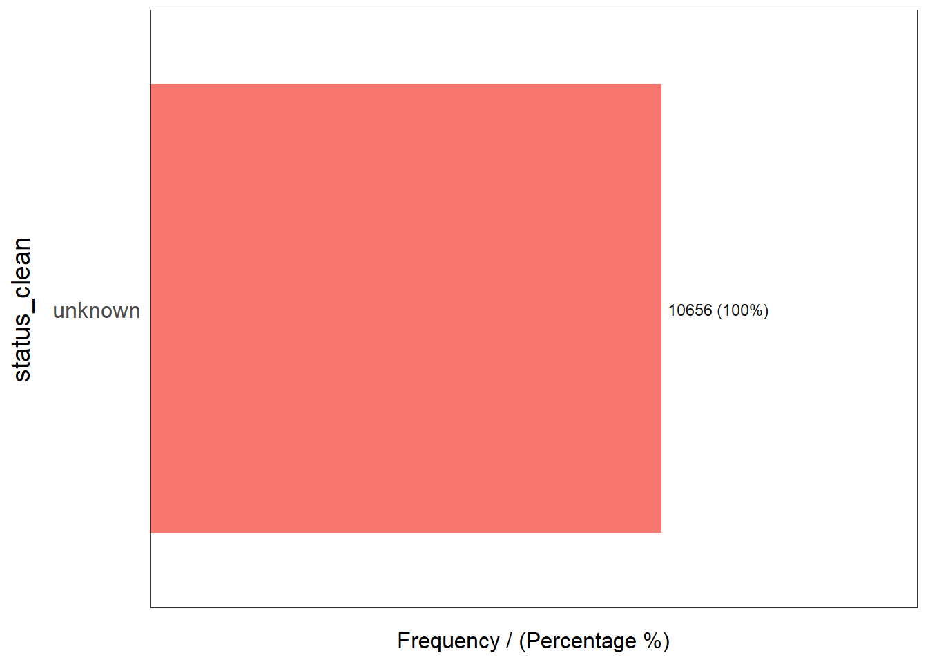

  status_clean frequency percentage cumulative_perc
1      unknown     10656        100             100

Performing Point-in Polygon Count

NGA_wp <- NGA %>%
  mutate(`total_wp` = lengths(
    st_intersects(NGA, wp_sf_nga))) %>%
  mutate(`wp_functional` = lengths(
    st_intersects(NGA, wp_functional))) %>%
  mutate(`wp_nonfunctional` = lengths(
    st_intersects(NGA, wp_nonfunctional))) %>%
  mutate(`wp_unknown` = lengths(
    st_intersects(NGA, wp_unknown)))

Visualising attributes by using statistical graphs

ggplot(data= NGA_wp,
       aes(x = total_wp)) + 
  geom_histogram(bins = 20,
                 color="black",
                 fill="light blue") + 
  geom_vline(aes(xintercept=mean(
    total_wp, na.rm=T)),
              color="red",
              linetype="dashed",
              size=0.8) + 
  ggtitle("Distribution of total water points by LGA") + 
  xlab("No. of water points") + 
  ylab("No. of\nLGAs") + 
  theme(axis.title.y = element_text(angle = 0))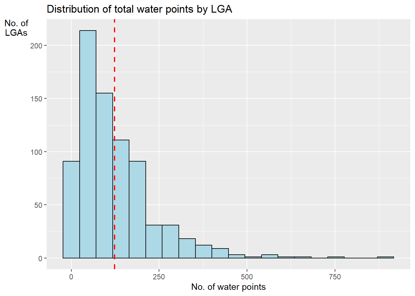

Saving the Analytical data in rds format

write_rds(NGA_wp, "data/rds/NGA_wp.rds")