In-Class Excercise 06

Published

February 18, 2023

Getting Started

Installing and Loading the required packages

pacman::p_load(tmap, sf, sfdep, tidyverse)

The Data

There are two datasets used for this exercise -

Hunan, a geospatial data set in ESRI shapefile format
Hunan_2012, an attribute data set in csv format

Importing Geospatial Data

hunan <- st_read(dsn = "data/geospatial", 
                 layer = "Hunan")

Reading layer `Hunan' from data source 
  `C:\mayurims\IS415-GAA\In-Class_Ex\In-Class_Ex06\data\geospatial' 
  using driver `ESRI Shapefile'
Simple feature collection with 88 features and 7 fields
Geometry type: POLYGON
Dimension:     XY
Bounding box:  xmin: 108.7831 ymin: 24.6342 xmax: 114.2544 ymax: 30.12812
Geodetic CRS:  WGS 84

Importing Attribute Table

hunan2012 <- read_csv("data/aspatial/Hunan_2012.csv")

Combining both data frame by using left join

Combine the Geospatial and Aspatial data here. One is a sf data frame and the other is a tibble data frame. One has a geometry column frame and the other doesn’t. If you want to retain the geometry column, then the left one should be the one with sf data frame and the right one should be the tibble data frame.

Notes :

Left_join() keeps all observations in x
Right_join() keeps all observations in y
Full_join() keeps all observations in x and y

Normally you need to join the unique identifier (common field), but in this case, we did not mention it. But here we can assume that it will find a field which is common. But we need to ensure that both have 88 observations and that the ‘County’ field name is same for both (the lower/upper case, etc.)

The select is just asking it to take the columns 1-4, 7 and 15 after they join. Because we just need these columns and the main - GDPPC. Hence, we drop the rest. If we don’t have the select function, we would have had 36 variables. We keep ‘NAME_3’ and ‘County’ for double checking.

hunan_GDPPC <- left_join(hunan, hunan2012) %>%
  select(1:4, 7, 15)

Plotting a Choropleth map

# You NEED this for Take Home Assignment 2!!
tmap_mode("plot")
tm_shape(hunan_GDPPC) + 
  tm_fill("GDPPC",
          style = "quantile",
          palette = "Blues",
          title = "GDPPC") + 
  tm_layout(main.title = "Distribution of GDP per capita by district, Hunan Province",
            main.title.position = "center",
            main.title.size = 1.2,
            legend.height = 0.45,
            legend.width = 0.35,
            frame = TRUE) + 
  tm_borders(alpha = 0.5) + 
  # tm_text("NAME_3", size=0.5) + 
  tm_compass(type = "8star", size = 2) + 
  tm_scale_bar() + 
  tm_grid(alpha = 0.2)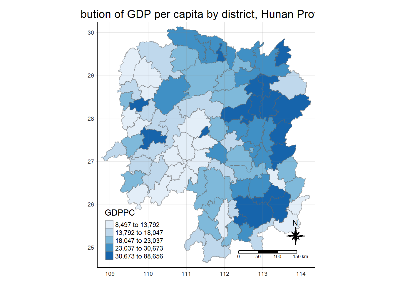

Identifying Area Neighbors

Before a spatial weight matrix can be derived, neighbors need to be identified first

Contiguity Neighbors Method

Default is Queen. The function poly2nb() used in Hands-on_Ex06 is the same as this function st_contiguity().

cn_queen <- hunan_GDPPC %>%
  mutate(nb = st_contiguity(geometry),
         .before = 1)

Here, when we make the queen = False, it becomes a Rook method. We do have another method called Bishop, but we don’t have it, since no one uses it.

cn_rook <- hunan_GDPPC %>%
  mutate(nb = st_contiguity(geometry),
         queen = FALSE,
         .before = 1)

K-Nearest Neighbors Method

Computing contiguity weights

Contiguity weights: Queen’s method

This code makes Contiguity Neighbors Method redundant as this code does that and combines the next code as well.

wm_q <- hunan_GDPPC %>%
  mutate(nb = st_contiguity(geometry),
         wt = st_weights(nb),
         .before = 1)

Contiguity weights: Rook’s method

wm_q <- hunan_GDPPC %>%
  mutate(nb = st_contiguity(geometry),
         queen = FALSE,
         wt = st_weights(nb),
         .before = 1)

Distance Band Method

This is for Fixed Distance criterion –> Lower limit has to be 0, so that the upper limit can be high!

Computing Contiguity Weights